LECTURE NOTES: Lessons from Simulating a Malthusian Economy
Uses of math, & limits of knowledge... Attempting to solve the C.P. Snow "two cultures" problem... The systemic parts of a Malthusian economy are (a) stagnant living standards, and (b) population...
Aha! SubStack now has a LATEX module!
And this makes me think, once again, that I should worry the question of C.P. Snow’s The Two Cultures in my economic history courses…
Basically, the 1/3 of students who take my economic history courses who come from economics, and from the STEM departments can and do use words to think—although perhaps not at the level that I would wish them to be able to. But the 2/3 of students who come from non-economics social science and humanities departments by and large cannot, do not, use numbers and algebra to think. For them, numbers, algebra, calculus, statistics, and so on are arcane ritual stumbling blocks, where sometimes they can learn to mouth the proper responses, but are by and large obstacles to understanding.
I keep thinking that there ought to be a way to shift this—and to teach the humanities and non-economic social-science majors some data science as well. (It seems to me quite likely that data-science knowledge and expertise is likely for our students to be much the same thing that being able to write a fine chancery hand was for a mediæval clerk, in terms of opening-up career and hence life possibilities.)
But how?
So here is a draft of a two-part lecture segment: one part on what economic models are, and a second trying to use an economic model to draw some conclusions—in this case, conclusions about the working of pre-modern Malthusian economies, “Malthusian” coming from the Rev. Thomas Robert Malthus, and his 1798 Essay on the Principle of Population:
Economic Models: What Are They Good For?:
In spite of the political complications, the nonexperimental nature, and the peculiar problems of cause and effect, economics is a quantitative science because most of the relationships that economists study come quantified. Thus economics makes heavy use of arithmetic and algebra, while political science, sociology, and most of history do not—save for statistics. .
The American economy is complex: 150 million workers, 12 million firms, and 100 million households buying and selling $24 trillion worth of goods and services per year. Economists must simplify it to understand this and other complex phenomena. So they restrict their attention to (a) some definitions, (b) a few behavioral relationships—cause-and-effect links between economic quantities—and (c) a handful of equilibrium conditions—conditions that must be satisfied for the state of the economy along some dimension to be relatively stable. They attempt to capture these behavioral relationships and equilibrium conditions in simple algebraic equations and geometric diagrams. Then they try to apply their equations and graphs to the real world, hoping their simplifications have not made the end-product of this “building the model” a distorted and faulty guide.
Just after the end of WWII Paul Samuelson of MIT discovered that many of his students were much more comfortable manipulating diagrams than solving algebraic equations. With diagrams, they could see what was going on in a hypothetical economy. Thinking of how a particular curve would shift was often easier than thinking of the consequences of changing the value of the constant term in an equation.
If you find analytic geometry easy and intuitive, then Samuelson’s intellectual innovation will make macroeconomics more accessible to you. Behavioral relationships become curves that shift about on a graph. Conditions of economic equilibrium become dots where curves describing two behavioral relationships cross (and thus both behavioral relationships are satisfied). Changes in the state of the economy become movements of a dot. Understanding economic theories and arguments becomes as simple as moving lines and curves around on a graph and looking for the place where the correct curves intersect. And solving systems of equations becomes easy, as does changing the presuppositions of the problem and noting the results. The equations, the graphs, and the descriptive words reinforce and shed light on each other.
But if you do not find analytic geometry easy and intuitive, then you are in trouble…
When economists are trying to analyze the implications of how people act they almost always write an equation that represents a behavioral relationship: how people respond to such-and-such a situation. This behavioral relationship states how the effect (the total level of production) is related to the cause (the available capital stock). The economist usually draws a diagram to help visualize the relationship, and also writes it down verbally: “A larger capital stock means that the average employee will have more machines and equipment to work with, and this will increase total production per worker. But increases in capital will probably be subject to diminishing returns to scale, so the gain in production from increasing the capital stock per worker from $40,000 to $80,000 will be less than the gain in production from increasing the capital stock per worker from $0 to $40,000.”
In addition to analyzing behavioral relationships, economists consider equilibrium conditions — conditions that must be true if the economy is to be in balance. If an equilibrium condition does not hold, then the state of the economy must be changing rapidly, moving toward a state of affairs in which the equilibrium condition does hold.
This model-building is a powerful way of thinking, if the details that you omit are indeed unnecessary, and if the factors emphasized are the most important factors.
Algebraic equations are the best way to summarize cause-and-effect behavioral relationships in economics. Because so many economic concepts are easily quantified, arithmetic might seem a more natural choice, but arithmetic quickly reaches its limits. For example, to know what the level of output per worker would be for each of a great number of possible levels of the capital stock per worker and the efficiency of labor, you would need to carry around a huge table. Table 3.2 shows just a tiny part of what would be required. It is much better to remember and to work with a single algebraic equation, like this one:
Algebra, moreover, has another advantage. It allows us to think about the consequences of a host of different possible systematic relationships by replacing the fixed and known coefficients that apply to only one situation with unspecified and potentially varying placeholder parameters. Using algebra to analyze this single equation allows us to manipulate and analyze all at once, in shorthand form, all the systematic relationships corresponding to different parameter values and all the tables that they summarize. And it is then easy moving back to the specific, when you want to consider a particular case with a particular set of values for the parameters.
Economic Modeling:
So with all that throat-clearing in the past, let us go to work:
Modeling & Simulating a Malthusian Economy:
Write down a very simple economic model for our pre-modern Malthusian economy. It will have four equations.
The first and second equations are simply definitions:
The first says that the proportional growth rate of living standards and productivity levels—the proportional growth rate of the output per worker y variable on the left-hand side—is equal to g, g for growth. The second says that the proportional growth rate of population and the labor force variable L, L for labor, on the right-hand side is equal to n, n for numbers.
The third and fourth equations are behavioral relationships:
The third says that g—the proportional growth rate of living standards and productivity levels—on the left-hand side is equal to the proportional rate of growth h of human ideas about technology, minus the proportional rate of growth of population and the labor force n divided by a parameter ɣ that tells us how salient ideas about technology are in generating productivity vis-à-vis resource scarcity. It is human ingenuity versus resource scarcity. And resource scarcity is made more dire by population increases.
The fourth says that the population growth rate variable n on the left-hand side will be such that population will grow if living standards y are above, and shrink if living standards are below, some “subsistence” level y^{sub}. It says that population will do so linearly, depending on a parameter β that tells us how responsive fertility and mortality are to want and deprivation. Twice as big a gap between living standards and subsistence will produce twice as fast a population response, with the value of the β parameter calibrating how much. As people get poorer, fertility drops: women become sufficiently skinny that ovulation becomes hit-or-miss. And as people get poorer, mortality rises: it is not just that some people starve to death, it is that the malnourished have compromised immune systems, and malnourished children, especially, are easily carried off by the common cold.
This model captures three features of the pre-modern economy:
There is (slow) progress in technology
A more prosperous society has higher population growth
Resource scarcity matters
What consequences do those features have?
Well, let us set up a toy economy—a simulation—with these features, and only these features, and see how history evolves. Let us set h = 0.0005—5% growth in technology over a century. Let us set β = 0.25—if real living standards are 40% over “subsistence”, population grows at 1% per year, or doubles in three generations. And let us set ɣ = 2—ideas about technology are twice as salient as resources in generating productivity. And we also need to add a random term, an ε term, for plagues, bountiful harvests, mild winters in which babies do not die of pneumonia, and all the other non-systematic accidents that affect the growth of population.
We could do this in Excel. We should not. Do anything even moderately complicated in excel, and you guarantee that you will make mistakes that you then will be unable to find and correct.
We will do this in Python—because it is easy, it is powerful, and it leaves a clear audit trail. You can skip the mechanics of the programming if you wish. Or you can work through them—either reading them, or creating your own Python Jupyter Notebook installation somewhere and programming it up.
A Simple Matter of Programming:
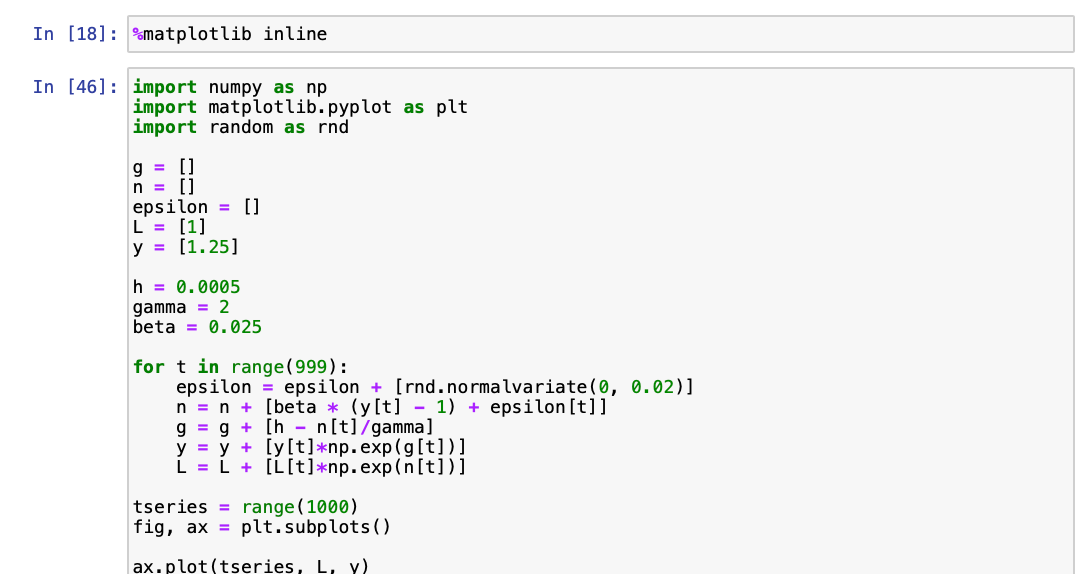
Go to <http://datahub.berkeley.edu> and create a new Python notebook file. Then we set up our simulation:
We want it to draw graphs in the main notebook file, not in separate windows.
We want to import three sets of commands and capabilities on top of the bare minimal Python installation—numerical Python, Python plot, and random numbers.
Then we are going to tell Python that it is going to have to keep track of five lists of numbers—the list of productivity growth rates g, of population growth rates n, of the labor-force level L (with L starting out at a benchmark index level of 1), of the productivity level y (with y starting out 25% above the subsistence level y = 1), and the list of random shocks to population ε.
We tell it what the values are of the technology-growth parameter h the ideas-salience parameter ɣ, and the population responsiveness parameter β.
Then we set up a loop to see what happens to our simulated society for 1000 years, populating the n, g, L, and y lists with the values they take on in each year in this run of the simulation.
Then we graph our variables—prosperity and population against time, and prosperity against population:
Pythonistas may well groan at this point: This code cell looks like it was badly translated from the FORTRAN. (FORTRAN, for “formula translator”, is a programming language that is now seventy years old.)
That is true: it is.
I can barely program any other way.
Pythonistas will say that there are more elegant, more concise, and more comprehensible ways of doing the job. And they are right. But in the words that Alfred Lord Tennyson puts in the mouth of his character Ulysses: “What we are, we are…”
Simulation Results:
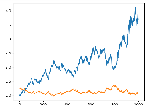
Here is where those of you who skipped the programming should come back. Here is one sample run from our simulation—graphs of simulated population and productivity over 1000 years:
The first graph plots time on the horizontal axis. On the vertical axis is the population of our simulated society over 1000 years, starting at an initial index value of 1, in blue; and also on the vertical axis is the productivity level of the economy over 1000 years, starting at an initial value 25% above the 1.0 benchmark of “subsistence” at which population is stable. Population grows erratically, because of the random shocks, but substantially over 1000 years. The economy’s productivity level does not: it stays near one, and pretty much all you can say is that productivity is relatively high after an extended period of population stagnation or decline, and low after an extended period of faster-than-average population growth:
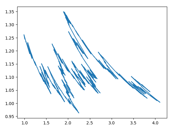
And here is productivity on the vertical axis plotted against population on the horizontal axis. In terms of time, the (population, productivity) pair for the economy is initially in the upper-left corner of the figure: at (1.0, 1.25). It then swings down and to the right and back up and to the left, all the while slowly moving right as technological knowledge accumulates:
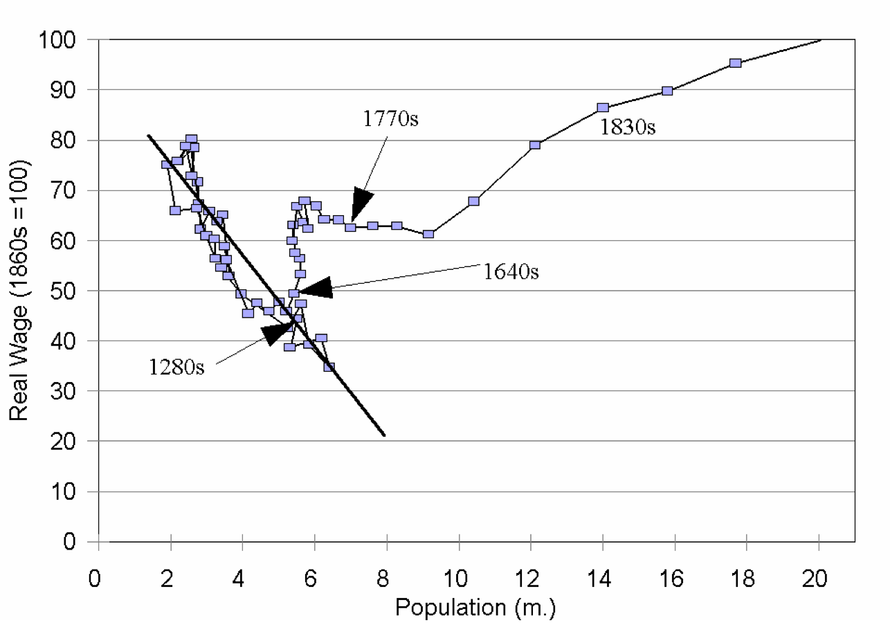
Does this not remind you of what we know about British population and wages from the medieval era up through 1700 or so? From Greg Clark’s The Condition of the Working Class in England:
After 1700 different processes were going on in English economy and society. But up to 1700, the family resemblance is clear. On average across the centuries the economy’s (population, productivity) point moves to the right, as technological progress (slowly) allows for a larger population to subsist in England. In a shorter but still substantial run, plagues and other demographic catastrophes cause the economy’s point to swing up and to the left, with a smaller population associated with higher productivity levels; and then down and to the right, as better living standards allow population to grow—and productivity decreases in response as resources per worker become scarce.
Lessons to Be Drawn:
One could take our simulation and write a history of different ages for it, searching for causes of the initial 250 years in which population doubles (and living standards decline), followed by 550 years of intermixed plague and other catastrophe-driven demographic decline and slow population growth, but with productivity and living standards ending that 550-year period at a level in the year 800 40% above their year-250 nadir. That age was then followed by another demographic boom in which the population doubles in 200 years.
No doubt stories about institutions, dynasties, cultures, and pathogens would play major and colorful roles in such a history. But when we look back at the guts of the simulation, we see that it is all chance: every year population and productivity are shifted not just by their structural determinants in the behavioral relationships, but by a random factor unconnected and uncorrelated with anything that has happened before, is happening now, or will happen later on.
This should give you pause: We are pattern-finding minds, and we find patterns even when they are not really there. It is not the case that shifting institutions, cultures, pathogens, and dynasties are driving the evolution of population and productivity in this simulation. Rather, the only forces systematically at work are:
The slow growth of technology at rate h, and thus the slowly growing ability of the economy to support more people at the same living standards.
The oscillations, or societal respiration as English-Ukrainian-Jewish mediæval economic historian M.M. Postan would say, as a series of past shocks that have generated a productivity level much higher than subsistence are then followed by relatively rapid population growth (and a decline in productivity and living standards), while favorable demographic shocks that have generated a relatively high population and low living standards are followed by population decline or stagnation (and a rise in living standards).
As I said: This exercise should give you pause. There may be nothing more to explain once one has understood the drift and respiration of a Malthusian economy, even if your pattern-solving East African Plains Ape mind strongly thinks that there must be something more than simply time and chance happening to them all.
If we were to eliminate all of the random shocks from our simulation, we would find that the economy in it, over time, would converge to a Malthusian steady-state path, along which:
Population and the labor force would grow just fast enough that increasing resource scarcity over time would offset the potential benefits in terms of higher living standards flowing from better technology. The economy would settle at a constant level for living standards just enough above subsistence to generate the population growth that increases resource scarcity by enough to offset the (slow) technological progress. It is this Malthusian equilibrium—and the fact that if disturbances shift the economy’s (population, productivity) pair away from it, the economy will move back toward the Malthusian equilibrium—that is the systematic, and hence the knowable, part of this system. At least, that is the case for this simulation.


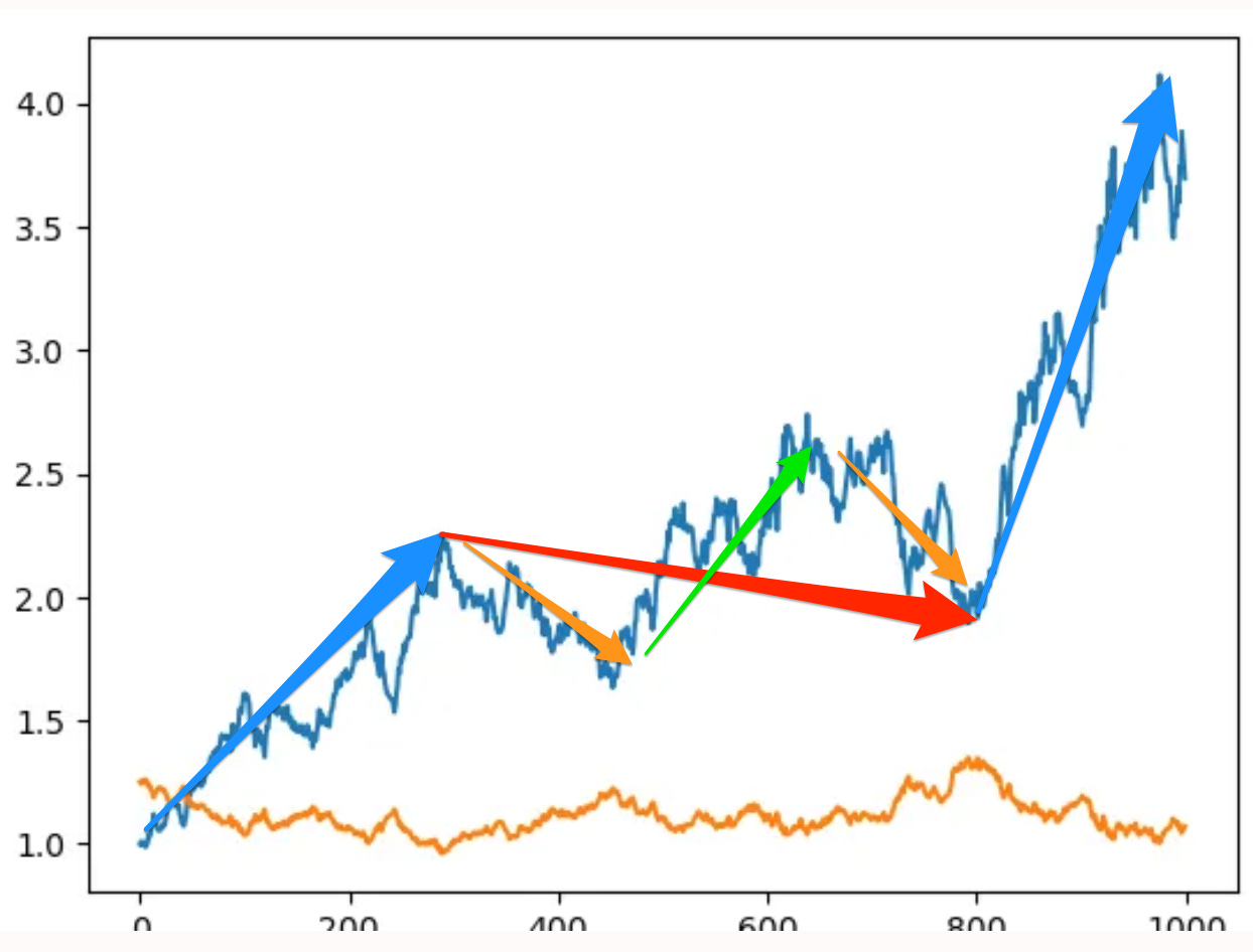
Dietrich Vollrath blogged a fantastic review of "Slouching" back in October (https://growthecon.com/feed/2022/10/11/DeLong-Review.html) in which he pointed out that to see 1870 as the "hinge of history" you really need to take into account the demographic transition. Your Python exercise above gave me the opportunity to visualize that perfectly.
Set the graph to have log scale on the y-scale (`ax.set_yscale('log')`) and at some arbitrary year (e.g. `t==500`) change h to 0.01:
Population starts to grow exponentially, but income bumps up by a small constant and then again becomes stagnant.
So to see the "hinge of history" we have to modify the equation for `n` in some way so that as income gets sufficiently high, `n` starts to fall.
Different topic, but has anyone else noticed that Tesla's quarterly US sales count isn't increasing? A company with a growth P/E that isn't growing, and is cutting prices.